02-solution

0001/01/01

${\bf 67}$ total marks.

Question 1 [10 points] A. Re-express the following small program using pipes.

c <- 18
f <- c*(9/5) + 32
print(f)
## [1] 64.4

f <- c %>% .[[1]]*(9/5) + 32
print(f)
## [1] 64.4

It’s pretty trick but just remember that whatever you pass through a pipe is called ${\tt .}$ and it’s actually a list. So if it is just a single item, it’s the first item in the list ${\tt .[[1]]}$

x <- 1e10
y <- sqrt( factorial(x) )
y <- x %>% factorial %>% sqrt %>% print
## [1] Inf

x<-3; mu<-5; sigma <-7
nrm <- ( 1 / (sigma * sqrt( 2 * pi ))) * exp( -(1/2) * ( (x - mu)/ sigma )^2)

p <- c(x = 3, mu = 5, sigma = 7)
p %>%
  { ( 1 / (.[["sigma"]] * sqrt( 2 * pi ))) * exp( -(1/2) * ( (.[["x"]] - .[["mu"]])/ .[["sigma"]] )^2 ) }
## [1] 0.05471239

So the trick is to combine the multiple parameters into a single vector first! That single vector is passed down the epipe.

p <- c( first = "a", second = "b", third = "c")

D. What is this equation?

Normal probablity distribution function.

site <- 15
gsub(";", "/", paste(paste( paste( "~hallett", paste("raw", "tara", sep = ";"), sep = ";"), 
      paste("site", site, sep="_"), sep=";"), 
      "dna_seq.fa", sep=";"))
## [1] "~hallett/raw/tara/site_15/dna_seq.fa"

site %>%
  paste("site", ., sep="_") %>% 
  paste("dna_seq.fa", sep=";") %>%
  paste("raw", "tara", ., sep = ";") %>%
  paste("~hallett", ., sep = ";") %>%
  gsub(";", "/", .)
## [1] "~hallett/raw/tara/site_15/dna_seq.fa"

The pipes makes this one a bit easier to read; do you agree?

Question 2 [5 points]

In total, how many black, african or asian women are included in the ${\tt small\_brca}$ dataset?

q2 <- small_brca %>% filter(gender=="FEMALE", race=="BLACK OR AFRICAN AMERICAN" | race=="ASIAN") %>%
  group_by(participant) %>% distinct %>% nrow
print(q2)

## [1] 249

Create a histogram of all asian individuals grouped by age. Each bar in the histogram should have two colours corresponding to male and females. (For example, red might be used for the fraction of women in some age group while blue is used for men in that same age group). Choose the number of bins (or binsize) in a way that makes your plot informative.

small_brca %>%
  filter(race == "ASIAN") %>%
  distinct(participant, .keep_all = TRUE) %>%
  mutate(age_at_diagnosis = as.numeric(age_at_diagnosis)) %>%
  ggplot(aes(x = age_at_diagnosis, fill = gender)) +
  geom_histogram(binwidth = 5)

So there are no males that fit this criterion. That’s ok. Also, you could use ${\tt birth\_days\_to}$ but you should divide by 365 first and take the absolute value (to make it more readable). Which to use is a bit of an esoteric issue: are you interested in their age at diagnosis or at last followup appointment?

Question 3 [7 points]

How many participants are there? (Careful: not samples but participants.) Show code.

small_brca %>% .["participant"] %>% distinct %>% nrow

## [1] 1092

A non-tidy way to do this would be as follows:

unique(small_brca$participant) %>% length

## [1] 1092

Both are perfectly ok. Do you undestand why we use ${\tt nrow}$ above but ${\tt length}$ in the non-tidy version?

List all of the ${\tt participant}$ that have more than one sample. Show code.

num_multi <- small_brca %>% group_by(participant) %>% summarise(count=n(), tumor, ESR1) %>%
          filter(count > 1) %>% arrange(participant)

## `summarise()` has grouped output by 'participant'. You can override using the `.groups` argument.

num_multi %>% nrow %>% print

## [1] 238

For the participants identified in 4b, create a scatter plot with the tumor on the $x$ axis and the normal on the $y$ axis (as specified by the ${\tt tumor}$ variable in the tibble) with points representing the expression of gene ${\tt ESR1}$.

for_plot <- num_multi %>% select(-count) %>%
    pivot_wider(names_from = tumor, values_from = ESR1, values_fn=mean) %>% rename(tumor='TRUE', normal='FALSE')

ggplot(data = for_plot, mapping = aes(x = tumor, y = normal)) +
  geom_point()

## Warning: Removed 3 rows containing missing values (geom_point).

So that is some tricky coding! If you managed that, congratulations. Do you understand why the ${\tt values\_fn}$ is necessary? Here I have chosen the ${\tt mean}$ (average) to combine when a patient has more than one normal or tumor samples. In such a dataset, can you suggest why it might be advantageous to have more than one sample for tumor or normal for a patient? I included the ${\tt arrange}$ and ${\tt rename}$ calls just to make things a bit more readable; they aren’t strictly necessary.

Question 4 [23 points]

Show your code for each step below.

When I made the assignment, I had intended to put this question as Question 2. I was a bit sloppy. It should be easy by now!

Part a [1 point] Load the ${\tt tidyverse}$ library and load the ${\tt small\_brca}$ dataset.

Part b [1 point] Write code that determines the number of rows (observations) and columns (variables) in ${\tt small\_brca}$.

Part c [1 point] Write code that displays the column names (names of variable) for columns $21$ to columns $24$ inclusive.

Part d [2 points] What is the mean expression level of FOXC1?

Part e [3 points] How many samples are there with FOXC1 expression levels above $245$?

Part f [5 points] Create a new tibble called ${\tt bw}$ that contains only those rows (observations) from ${\tt small\_brca}$ that correspond to tumor samples of BLACK OR AFRICAN AMERICAN women.

Part g [5 points] Using ${\tt small\_brca}$, select the variables ${\tt participant}$, ${\tt vital\_status}$, and all genes except ${\tt RRM2}$.

Part h [5 points] Create a new variable called ${\tt triplenegative}$ in the tibble ${\tt small\_brca}$ that is TRUE (logical) if the sample is “Positive” for ${\tt er\_status\_by\_ihc}$, and not “Positive” for ${\tt her2\_fish\_status}$. Otherwise, in all other cases it is FALSE.

#a
library(tidyverse)  # dont' need to install it; it's already been installed by MH
load("~/data/GDC/TCGA_BRCA/small_brca.Rdata") 

#b
(dim(small_brca)) # one way to do it.

## [1] 1215   79

(nrow(small_brca))

## [1] 1215

(ncol(small_brca))

## [1] 79

#c
colnames(small_brca)[21:24]

## [1] "er_status_by_ihc"               "er_status_ihc_Percent_Positive"
## [3] "pr_status_by_ihc"               "pr_status_ihc_percent_positive"

#d
small_brca %>% summarize( my_mean= mean(FOXC1, na.rm=TRUE) ) %>% .[['my_mean']] %>% print

## [1] 1717.955

#e 
small_brca %>% filter( FOXC1 > 245 ) %>% nrow

## [1] 909

#f 
bw <- small_brca %>% filter( race=="BLACK OR AFRICAN AMERICAN", gender=="FEMALE", tumor==TRUE  )

#g 
small_brca %>% select( participant, vital_status, ANLN:TMEM45B ) %>% select( -RRM2 )

## # A tibble: 1,215 x 51
##    participant vital_status  ANLN FOXC1  CDH3 FGFR4 UBE2T NDC80   PGR BIRC5
##    <chr>       <chr>        <dbl> <dbl> <dbl> <dbl> <dbl> <dbl> <dbl> <dbl>
##  1 A1NF        Alive         2124   235   485   261  1002  1184   710  1242
##  2 A27M        Alive         4679  2068 15686   150   634   856    99  3429
##  3 A0GZ        Alive         1192   284  3999   171  1314   732  8793  1738
##  4 A18V        Dead         10191  2981 27406   473  1720  1853    76  4542
##  5 A13G        Alive          823   142   435    46    77    45  8804   152
##  6 A275        Alive        10198   265  6903  8835  2997  1887    76  5517
##  7 A0XS        Alive          669   294  1407   159   305   352 57567   673
##  8 A5RW        Alive         1342  5638  2975   195  2275  2572    12  5022
##  9 A5RX        Alive          420   531  5030   327   509   122 19520   284
## 10 A1RD        Alive         1124   189   299   649   679   550 21586   982
## # … with 1,205 more rows, and 41 more variables: ORC6 <dbl>, ESR1 <dbl>,
## #   PHGDH <dbl>, PTTG1 <dbl>, MELK <dbl>, NAT1 <dbl>, CXXC5 <dbl>, BCL2 <dbl>,
## #   GPR160 <dbl>, EXO1 <dbl>, UBE2C <dbl>, TYMS <dbl>, KRT5 <dbl>, KRT14 <dbl>,
## #   MAPT <dbl>, CDC6 <dbl>, MMP11 <dbl>, MYBL2 <dbl>, SFRP1 <dbl>, CCNE1 <dbl>,
## #   BLVRA <dbl>, BAG1 <dbl>, MLPH <dbl>, CDC20 <dbl>, CENPF <dbl>, MIA <dbl>,
## #   KRT17 <dbl>, FOXA1 <dbl>, ACTR3B <dbl>, CCNB1 <dbl>, MDM2 <dbl>, MYC <dbl>,
## #   CEP55 <dbl>, SLC39A6 <dbl>, ERBB2 <dbl>, GRB7 <dbl>, KIF2C <dbl>,
## #   NUF2 <dbl>, EGFR <dbl>, MKI67 <dbl>, TMEM45B <dbl>

#h within the tidyverse

small_brca <- small_brca %>% mutate( triplenegative = ifelse(er_status_by_ihc=="Positive",  TRUE , FALSE    ) )

#h - non-tidy verse way
small_brca$triplenegative <- ifelse(small_brca$er_status_by_ihc=="Positive",  TRUE , FALSE    )

Note that when I work on my machine at home, the path is different. Your path for the ${\tt load}$ should look something like $data/small_brca.Rdata$ because you are on RStudio Cloud and your directory structure looks the same. That’s one of the advantages of RStudio Cloud: you don’t need to struggle with paths on your own machine as much.

There are different ways to do part (d). For example, in a none-tidyverse way:

( mean( as.numeric(small_brca$FOXC1 ), na.rm=TRUE ) )

## [1] 1717.955

In both cases, do you understand the reason for ${\tt na.rm}$? Also, the ${\tt as.numeric}$ is necessary because when you use the ${\tt \$}$ to select a column, it is still a tibble (it’s just a single column tibble). You need to turn that tibble into a vector of numbers. Make sure you understand the ${\tt ifelse}$ function; it’s handy.

Question 5 [12 points]

Using the ${\tt small\_brca}$ tibble, create the following plot.

ggplot(data = small_brca) +  
  geom_point(mapping = aes(x = GRB7, y = EGFR, color=tumor)) + 
  facet_wrap(~ tumor_status, nrow = 2) +
  scale_y_continuous(trans='log')   + scale_x_continuous(trans='log') + 
  ggtitle("GRB7 and EGFR expression by tumor_status") +
  xlab("log GRB7 expression") +  ylab("log EGFR expression")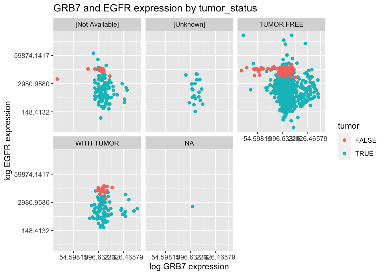

Question 6 [5 points]

The variable ${\tt race}$ in ${\tt small\_brca}$ has several different possible values including “WHITE”, “ASIAN”, “BLACK OR AFRICAN AMERICAN”, “AMERICAN INDIAN OR ALASKA NATIVE”, “[Not Available]”, “[Not Evaluated]”, or NA.

It is better to simply use NA instead of“[Not Available]”, “[Not Evaluated]”, or NA. It will simplify your code in downstream analyses.

Write R code to create a new ${\tt race\_modified}$ variable where all samples with “[Not Available]”, “[Not Evaluated]” are changed to NA (Note: you shouldn’t use “NA”, but NA. They are not the same)

print(unique(small_brca$race))

## [1] "WHITE"                            "ASIAN"                           
## [3] "BLACK OR AFRICAN AMERICAN"        "[Not Available]"                 
## [5] "[Not Evaluated]"                  NA                                
## [7] "AMERICAN INDIAN OR ALASKA NATIVE"

small_brca <- small_brca %>% mutate(race_modified = ifelse((race=="[Not Available]" | 
                                                             race=="[Not Evaluated]" |
                                                             race=="NA"), NA, race))
print(unique(small_brca$race_modified))

## [1] "WHITE"                            "ASIAN"                           
## [3] "BLACK OR AFRICAN AMERICAN"        NA                                
## [5] "AMERICAN INDIAN OR ALASKA NATIVE"

Question 7 [5 points] Pick one of the $50$ genes from ${\tt small\_brca}$ uniformly randomly (see the ${\tt runif}$ function). Using the NCBI, provide the following information or note that it is not availalbe:

colnames(small_brca)[runif(1, min=37, max=79)] %>% print

## [1] "TYMS"

The rest of the answers for Question 7 are specific to the invividual.

10a Full name of the gene and the official name according to the HGNC.
10b First time it was reported in the literature.
10c Where it is located in the genome.
10d Its ${\tt gi}$ acccession code or codes (if it has been modified).
10e The number of exons.
10f The number of alternative transcripts that have been record.
10g Its full amino acid sequence. Provide its protein ID.
10h Its protein structure, if known.